神经退行性病
-
Figure 1|Patient flow chart.
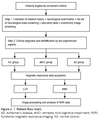
We excluded patients with a Hachinski ischemic index score (Pantoni and Inzitari, 1993) of 4 or more, hypothyroidism, vitamin B12 or folic acid deficiency, a long history (more than 5 years) of smoking and alcohol abuse, inability to complete an MRI scan (patients with contraindications to MRI scanning, i.e., severely febrile, critically ill, claustrophobic, in early pregnancy, and with metal implants in the body or metal foreign bodies) or neuropsychological testing, traumatic brain disease or a history of other brain disorders, Parkinson’s syndrome, epilepsy, and those with other systemic neurological disorders that severely affect cognitive function and systemic disorders that can affect MRI scans or neuropsychological tests. We excluded patients whose fMRI images failed visual quality control or pre-processing. The trial procedure is shown in Figure 1.
Figure 2|Process of dFCS calculation.
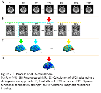
We used the DynamicBC toolkit (v1.1, www.restfmri.net/forum/DynamicBC) to calculate the global dFCS for each voxel with the sliding window approach, as shown in the flow chart in Figure 2. We set the length of the window to 50 repetitions with an overlap of 0.6. The rest of the parameters were identical to a previous study (Luo et al., 2019) (230 total repetitions were available and 7 windows were created.) For each window, we first calculated the global dFCS at each voxel as the sum of the functional connectivity between this voxel and the other voxels in the brain mask. We adopted the threshold P < 0.001 to eliminate voxels with weak correlations attributable to signal noise and removed negative correlations. Then, we obtained a series of dFCS maps corresponding to the number of windows. The variance of each dFCS map across time was calculated to measure its temporal variability. Finally, on the basis of a previous study, the variance of the dFCS map for each subject was transformed to a Z score by subtracting the mean values divided by the standard deviation of all values within the brain mask to control the global effects (Zou et al., 2008).
Figure 3|Five-fold cross validation.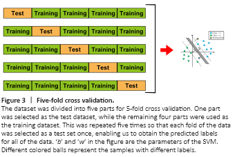
To discriminate aMCI and AD from NC, we used the variance of dFCS maps as features and trained linear SVM models using LIBSVN 3.25 (https://www.npackd.org/p/libsvm/3.25). This led to a model with more interpretability than other non-linear models and less susceptibility to over-fitting. Because of the limited study population, we used 5-fold cross validation (Figure 3) to evaluate the performance of the models. In each model, four-fifths of the participants were selected as the training dataset, and the other participants were used as the test dataset. Because the classification was pair-wise, we used a two-sample t-test to select the features with P values < 0.05 in the training dataset. Although they can preserve multivariate patterns, we did not use multivariate feature selection methods such as recursive feature elimination because they are time-consuming. Before inputting the data into the model, we normalized the features using the mean values and standard deviations from the training dataset. We used the accuracy, sensitivity, specificity, area under the curve, positive predictive value, negative predictive value, and F-score to evaluate model performance. We used the permutation test to determine whether the obtained final metrics were significantly better than chance. Specifically, we ran the above prediction procedure 1000 times. For each time, we permuted the labels across the samples without replacements. The P values of the metrics were calculated by dividing the number of permutations with a higher value than the actual value for the real sample by the total number of permutations. For each sample, we also calculated the decision value, which is the distance between the samples on a hyperplane that is determined by SVM classifiers. We also used partial correlation analysis to explore the relationship between decision values and MMSE and MoCA scores.
Figure 4|The difference in dFCS among the NC, aMCI, and AD groups.
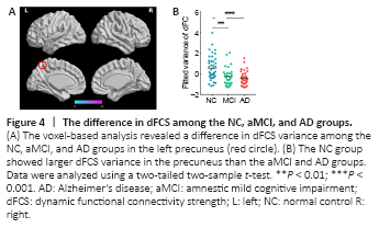
Using voxel-wise analysis, we found significant differences in dFCS variance in a cluster including the left precuneus among the three groups (Figure 4A). The Montreal Neurological Institute coordinates of the peak voxel, which had an F value of 12.03, were (–3, –60, 57) and the cluster size was 6. Then, we extracted the mean variance of the dFCS in the left precuneus. A two-tailed two-sample t-test (Figure 4B) showed that the mean variances of the dFCS in the left precuneus region of patients with aMCI (P < 0.01) and AD (P < 0.001) were lower than that in the NC group.
Figure 5|Correlations between the mean dFCS variance in the precuneus with MMSE (A) and MoCA (B) scores.
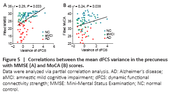
A partial correlation analysis controlling for sex, age, and education revealed that the mean variance of the dFCS in the left precuneus was significantly positively correlated with MMSE (r = 0.29, P = 0.003) and MoCA (r = 0.24, P = 0.038) scores (Figure 5).
Figure 6|Correlations between decision value and MMSE (A) and MoCA (B) scores.
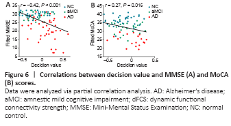
We performed a partial correlation analysis to explore whether the decision values generated from the SVM classifiers were correlated with the MMSE and MoCA scores. As shown in Figure 6, the decision values were significantly correlated with the MMSE (r = 0.42, P < 0.001) and MoCA (r = 0.27, P = 0.016) scores.
Figure 7|The weight of classifying the aMCI from the NC group.
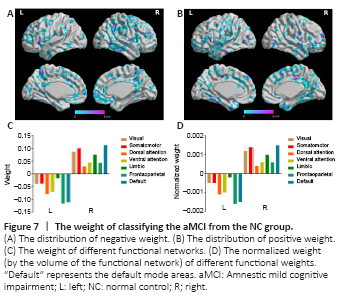
Figure 8|The weight of classifying the AD from the NC group.
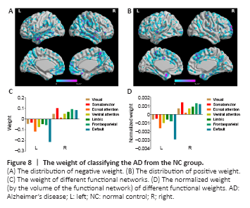
We also considered the mean positive and negative weights in the brain networks (Yeo et al., 2011). In the aMCI-NC classifier, the DMN and frontoparietal network were the most contributive networks (Figure 7), whereas in the NC-AD classifier, the weights were almost all negative and mainly located in the DMN (Figure 8). For both the aMCI-NC and AD-NC classifiers, the visual network, somatomotor network, ventral attentional network, and limbic network had positive weights, with two clear phenomena. First, the weight of the positive contribution of the above networks was significantly higher in the aMCI-NC group than in the AD group. Second, the contribution weight of the somatomotor network was mainly positive, and its weight was second only to that of the DMN.