神经损伤与修复
-
Figure 1|Tissue processing steps for optical clearing.
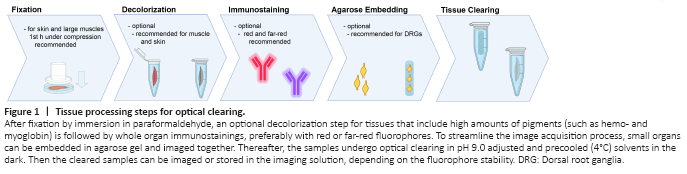
Investigators rely heavily on the quantification of regenerated motor and sensory neurons following experimental nerve repair to evaluate the extent of nerve regeneration. However, conventional tissue sectioning is labor intensive, susceptible to cutting artifacts, and requires correction factors to estimate the true number of neurons (Abercrombie, 1946). To overcome these challenges, we used a modified FDICSO protocol to clear intact spinal cord and entire dorsal root ganglia (DRGs) of adult rats and to quantify fluorescently labeled neurons via automated image segmentation (Figure 1).
Figure 2|Neuron segmentations in the optically cleared spinal cord and dorsal root ganglia.
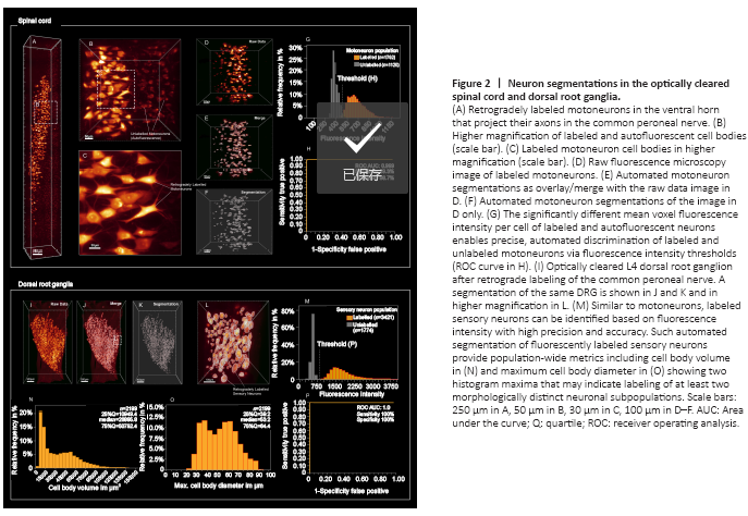
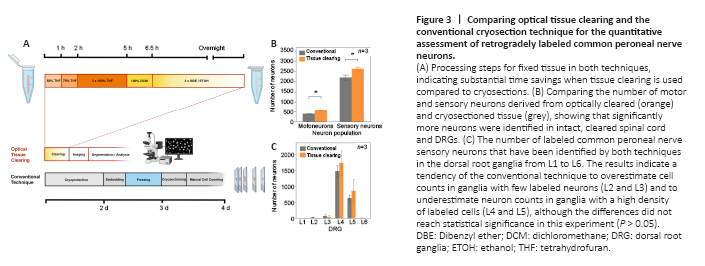
Figure 3| Comparing optical tissue clearing and the conventional cryosection technique for the quantitative assessment of retrogradely labeled common peroneal nerve neurons.
Using immersion in a series of commercially available solvents, we achieved almost complete transparency for both, spinal cord and DRGs within 24 hours (Figures 2 and 3). Thereafter, the immersed specimens were imaged via fluorescence microscopy. We found light-sheet microscopy to be best suited to large, cleared tissue specimens, due to the rapid image acquisition, minimal photobleaching, and high spatial resolution (Figure 2A–C).
Figure 4|Filament tracing in optically cleared peripheral nerve and skeletal muscle.
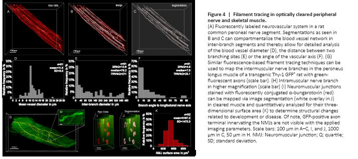
Sufficient blood supply is essential to clear debris and establish a pro-regenerative environment following peripheral nerve injury. Accordingly, ischemia has been described as a determining pathomechanism in neuropathies and a key length-limiting factor for acellular nerve allografts and synthetic conduits (Best et al., 1999; Ostergaard et al., 2015; Goncalves et al., 2017). However, the historically challenging assessment of the neurovascular network in three dimensions has been a limiting factor for conclusive morphological studies. We used optical tissue clearing techniques to render peripheral nerve segments transparent and thereby make the intraneural vascular network accessible for high-resolution fluorescence microscopy (Figure 4A). In specimens harvested from animals that did not undergo transcardial perfusion, vessels still contained red blood cells which are intensely autofluorescent in the green emission spectrum. This can already be used as a broad approximation to map larger blood vessels, but in smaller capillaries, we found the distribution of red blood cells to be inconsistent. We therefore used an intravenous injection of fluorescently conjugated CD31 antibody to label the endothelial walls of the entire vascular network. Using a far-red emission spectrum, we obtained consistent staining across upper and lower extremity peripheral nerves. Automated blood vessel tracing based on fluorescence intensity thresholds enabled mapping of the neurovascular network including capillaries with an inner diameter below that of red blood cells (< 6 μm) as shown in Figure 4B–D. Beyond visualization and qualitative assessment, we were able to segment the blood vessels in inter-branch segments for detailed quantitative analysis. Exemplary, we segmented a 1000 μm segment of a rat common peroneal nerve (Figure 4). The inner diameter of the intraneural blood vessels ranged between 4.0 μm and 23.5 μm, averaging 11.6 ± 3.3 μm (Figure 4D). Most inter-branch segments were short (< 40 μm), but some blood vessels spanned over almost 400 μm between two branch points (Figure 4E). When analyzing the angle between the vascular axis and the longitudinal nerve axis, the blood vessels were predominantly longitudinally oriented, as previously described (Best and Mackinnon, 1994). However, approximately 5% of the inter-branch segments were orientated perpendicular to the nerve axis, representing perforators that connect epi- and perineural to endoneurial blood vessels (Figure 4F).
Transparent skeletal muscles allow for comprehensive analysis of intramuscular neuronal projections and their neuromuscular junctions. This may be used to quantitatively assess the re-innervation process following peripheral nerve repair or determine disease-related changes in the neuromuscular architecture. We used threshold-based filament tracing to visualize motor nerve branches within a peroneus longus muscle of a Thy-1 GFP+ rat, a commonly used target muscle for experimental nerve repair studies (Figure 4G and H). Notably, PFA fixed skeletal muscle features a pronounced autofluorescence in the green and red emission spectrum (Figure 4H), making far-red the preferred fluorophore for muscle imaging due to a higher signal-to-noise ratio, as previously described (Williams et al., 2019). To visualize the NMJs, we intravenously injected α-Bungarotoxin conjugated with a fluorescent marker in the far red-spectrum (Chen et al., 2016). Similar to principles of transcardial perfusion, tail vein injections use the blood flow to distribute the conjugated antibody evenly throughout the entire system. Thereby, the injections rapidly achieve homogenous stainings of intact muscles that are otherwise difficult for antibodies to penetrate with post-mortem immunohistochemistry (Chen et al., 2016). Homogenous NMJ stainings can be confirmed after tissue clearing. NMJ morphology is remarkably stable in rodents with intact nerves (Balice-Gordon and Lichtman, 1990). In response to denervation or reinnervation, however, NMJs undergo substantial structural reorganization and change their appearance and surface area (Rich and Lichtman, 1989). Such metrics can be precisely quantified on a large scale in optically cleared skeletal muscle. To demonstrate their applicability, we randomly segmented a region of interest measuring 0.5 × 0.5 × 1.0 mm3 within a rat peroneus longus muscle within which we identified a total of n = 52 separate neuromuscular junctions. Using the Imaris surface tool, we created surfaces with 0.3 μm surface detail for each NMJ to quantify the three-dimensional surface area (Figure 4I and J). The surface area of the physiologically innervated NMJ‘s ranged from 2840.3 μm2 to 9712 μm2 with an average area of 5167.2 ± 1475.3 μm2 (Figure 4K).
Figure 5|Cutaneous innervation in the rat sural nerve dermatome.
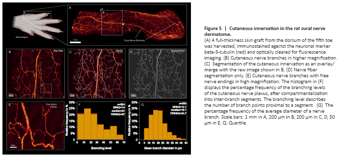
To determine the applicability of optical clearing techniques to assess skin innervation, we harvested full-thickness skin flaps from the sural nerve dermatome of adult Sprague Dawley rats. Immediately before harvest, we applied hair removal cream (Veet, Reckitt Benckiser, UK) to remove the strongly autofluorescent hairs. To facilitate imaging, we flattened the skin flaps with gentle pressure during the first hour of PFA fixation. Subsequently, the samples were decolorized, permeabilized, and immunostained against neuronal cell markers. Given the green autofluorescence and rapid, solvent-induced quenching of endogenous GFP expressed under the Thy-1 promoter in this rat model, we used additional immunostaining against beta-3-tubulin to improve signal-to-noise ratio. Using optical tissue clearing, the full-thickness skin flaps were rendered transparent and then imaged via confocal microscopy. Despite moderate autofluorescence in the red spectrum, the cutaneous nerve branches were clearly visible (Figure 5A and B). Within each nerve branch, individual axons were distinguishable that terminated in free- or lanceolate nerve endings in the skin and around hair follicles (Figure 5E). To quantitatively assess the cutaneous innervation, we segmented a region of interest of 2500 μm × 2000 μm (Figure 5B–D). The skin innervation density, defined as nerve branch length per region of interest area, was 9508.9 μm/mm2. Of note, this is 2.6-fold lower compared to the nerve fiber density in the cornea of the same rat strain (Catapano et al., 2018). The median branching angle of the cutaneous nerve fibers was 33.9° and the median branch length was 63.85 μm. We found 56 free nerve endings per mm2, some of which arose from nerve branches with more than 60 branching points within the region of interest, demonstrating the arborized architecture of the cutaneous nerve plexus (Figure 5F).